Summary
anomalous([<anomalousType>,]<testWindow>, [<confidenceFactor>,] [<historyWindow>,] <tsExpression>
[,boundaryOptions])
Returns the percentage of anomalous points in each time series described by the expression. Points are considered anomalous if their values fall outside an expected range, as determined by the given confidence factor.
Parameters
| Parameter | Description |
|---|---|
| anomalousType | Optional type of anomalies to focus on. Use low to focus on lower bound violations. Use high to focus on upper bound violations. By default, both low and high anomalies are shown. |
| testWindow | Length of the test window, which is the moving time window to check for anomalous points. You can specify a time measurement based on the clock or calendar (1s, 1m, 1h, 1d, 1w), the window length (1vw) of the chart, or the bucket size (1bw) of the chart. Default is minutes if the unit is not specified. |
| confidenceFactor | A number from 0.0 to 1.00 (inclusive) that expresses the confidence factor for determining the range of expected values. This number is used to compute the range as a number of standard deviations around the mean expected value. Default is 0.99 if this parameter is not specified. |
| historyWindow | Optional amount of time in the history window, which is the time window that immediately precedes the chart window. Default is 1 day (1d) if this parameter is not specified. Points in the chart window and the history window are the basis for computing the expected values in the test window. You can specify a time measurement based on the clock or calendar (1s, 1m, 1h, 1d, 1w), the window length (1vw) of the chart, or the bucket size (1bw) of the chart. |
| tsExpression | Expression describing the time series to inspect for anomalous points. |
| boundaryOptions | Determines whether confidence boundaries are show.
|
Description
The anomalous() function analyzes data points in the time series described by the expression, and returns the percentage of points that have anomalous (unexpected) values. Values are considered anomalous if they fall outside a range of expected values. By default, anomalous() uses a range that is predicted with 0.99 (99%) confidence.
anomalous() always returns results between 0 and 1. If there is no anomaly between the underlying values (all values are NaN), anomalous() returns all zeros.
anomalous() analyzes successive groups of data points in a time series, and returns the percentage of anomalous points for each group. You define the groups by specifying the testWindow parameter. For example, anomalous(10m, ts(my.metric)) returns, for each data point, the percentage of data points with anomalous values that were reported during the 10 minutes before that data point. If 4 out of 10 points in a test window have anomalous values, the result returned for that test window is 0.40.
anomalous() returns the result for a test window at the end of that window. Consequently, the longer the test window, the more the result might appear to be delayed after a sudden change in the time series. If you choose a short test window, the result will coincide more closely to the time series change. A typical test window is 10m.
anomalous() returns a separate series of results for each time series described by the expression.
You can specify optional parameters to anomalous() to adjust the range of expected values, or to fine tune the input values on which prediction is based.
Adjusting the Range of Expected Values
anomalous() uses a forecasting algorithm to predict a range of expected values for each data point reported in the chart for the time series. A reported data point is considered anomalous if its value falls outside of the range that is predicted for it.
The range of expected values for a point is organized in standard deviations around a mean expected value. You can adjust the width of the range by specifying a numeric confidenceFactor parameter. anomalous() uses this number to compute the number of standard deviations to include in the range. For example:
- Specify 0.99 to include 99% of the expected values in the range. Consequently,
anomalous(5m, .99, ts(my.metric))returns the percentages of points that fall outside 3 standard deviations from the mean expected values. (Note: This is the default, so omitting.99is the same as specifying it.) - Specify 0.95 to include 95% of the expected values. Consequently,
anomalous(5m, .95, ts(my.metric))returns the percentages of points that fall outside 2 standard deviations from the mean expected values. - Specify 0.68 to include 68% of the expected values. Consequently,
anomalous(5m, .68, ts(my.metric))returns the percentages of points that fall outside 1 standard deviation from the mean expected values.
If the range is narrow, many points lie outside it, and the reported percentages are large. If the range is wide, few points will lie outside it, and the reported percentages are small. The narrower the range, the more points might be considered anomalous, and the higher the reported percentages.
Tuning Value Prediction
anomalous() uses a forecasting algorithm that bases its predictions on actual values reported by the time series. These values come from data points reported in the chart window and data points reported in a history window immediately preceding the chart. In effect, the history window provides a minimum amount of past data for anomalous() to base its predictions on, regardless of the size of the chart’s time window.
By default, the history window is one day long. You can fine tune the forecast by adding an optional historyWindow parameter to specify a longer or shorter history window. A longer history window supports more accurate prediction, although the query might take longer.
For example, anomalous(5m, 2w, ts(my.metric)) predicts the expected values based on 2 weeks’ worth of actual data points in addition to the data shown in the chart.
Example
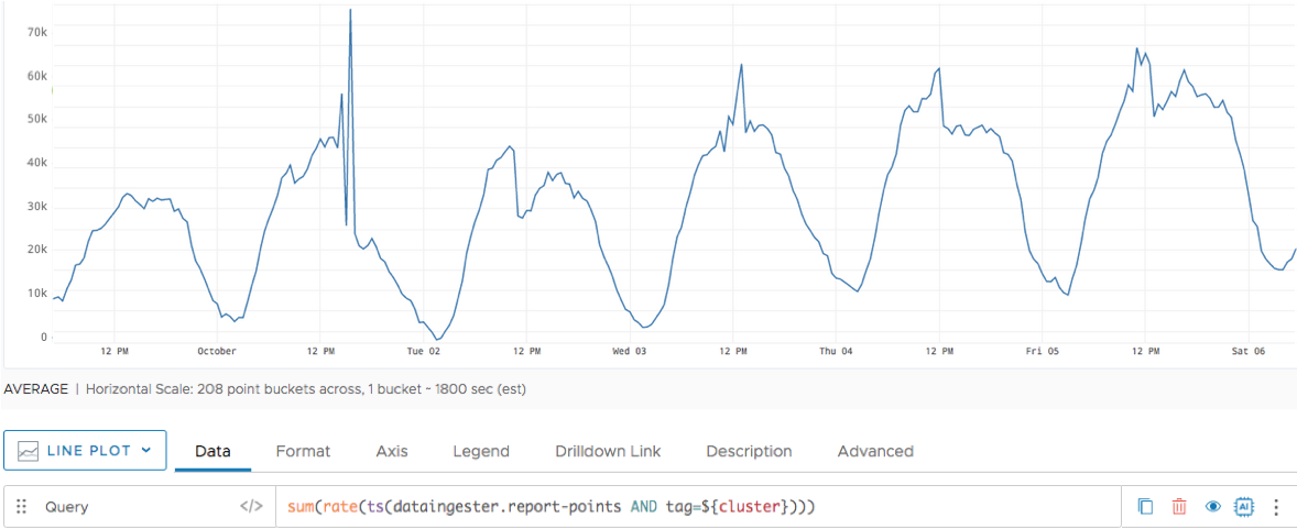
The following chart shows an aggregated rate of data ingestion for a particular cluster. Data ingestion appears to fluctuate daily, with lower rates around midnight and peaking around noon.
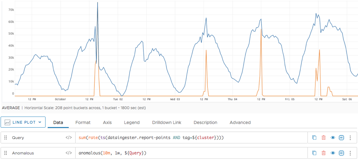
We’d like to know whether the actual fluctuation deviates from the expected fluctuation, based on about 2 weeks’ worth of actual data (the week before the chart and the week shown in the chart). We want to keep the test window short, to better correlate the results with the changes in the time series. So we run anomalous() with a 10m test window and a 1w history window.
The orange line in the following chart suggests that the spikes in data ingestion on the afternoons of October 1, 3, 4, and 5 may be anomalous because they fall outside the range of 99% of expected values. In contrast, the behavior on the afternoon of October 2 seems right in line with expectations – the percentage of anomalous points here is 0.
Using the anomalous() Function in Alerts
anomalous() function are resource intensive and need to be used carefully. Otherwise, they can cause high loading on the service.History Size and Test Window Size
When you use the anomalous() function in alerts, you must adjust some parameters. The most important ones are history window(historyWindow) and test window (testWindow).
To understand what’s the best value to use for historyWindow, you must answer the simple questions: What type of anomalies am I looking for? Am I interested in daily, weekly, or monthly anomalies?
After you decide what history window to use, you must select the test window. The test window value is based on the history window parameter, as those two parameters are interconnected. The ratio between the test window and history window is recommended to be more than 1:500, so if the selected value is too small to run the algorithm optimally, it will be tweaked by the system, and you’ll see the following warning message:
The ratio between history window and test window is not optimal and will result in bad performance. History window has been optimized to …
Alert Firing Window and Checking Frequency
To minimize the load on the system, you may want to tweak the Trigger Window window and Checking Frequency parameters based on the history window and the test window values that you choose.
You can set the Trigger Window window parameter under Condition and the Checking Frequency parameter when you click the Advanced link.
For optimal and effective execution of the alerts that are based on anomaly detection, update the default values for the Trigger Window window and alert Checking Frequency.
Choose an Trigger Window window based on the following equation:
Trigger Window = Test window / 10 * K, where K = 1, …, 10
Choose an alert Checking Frequency that is more than Test window/10, as the execution of the anomaly detection algorithm with lower values will take as an input the same historical duration, which will cause redundancy.