VMware Tanzu Observability (formerly known as VMware Aria Operations for Applications) supports histograms for computing, storing, and using distributions of metrics rather than single metrics. Histograms are useful for high-velocity metrics about your applications and infrastructure – particularly those gathered across many distributed sources. You can send histograms to a Wavefront proxy or use direct ingestion.
This page explain how to send histogram distributions. After the data is available, you can visualize histogram distributions using Histogram charts or Heatmap charts.
Getting Started
Watch this video for an introduction to histograms. Note that this video was created in 2018 and some of the information in it might have changed.
The following blog posts give some background information:
- What if I Told You Your Monitoring Data is Lying: Why Histograms are Critical for Accurate Reporting of Hi-Velocity Metrics
- How the Metric Histogram Type Works: True Visibility into High-Velocity Application Metrics
Why Use Histograms?
Tanzu Observability can receive and store highly granular metrics at 1 point per second per unique source. However, some scenarios generate even higher frequency data.
Suppose you are measuring the latency of web requests. If you have a lot of traffic at multiple servers, you may have multiple distinct measurements for a given metric, timestamp, and source. Using “normal” metrics, we can’t measure this because, rather than metric-timestamp-source mapping to a single value, the composite key maps to a multiset (multiple and possibly duplicate values).
One approach to dealing with high frequency data is to calculate an aggregate statistic, such as a percentile, at each source and send only that data. The problem with this approach is that performing an aggregate of a percentile (such as a 95th percentile from a variety of sources) does not yield an accurate and valid percentile with high velocity metrics. That might mean that even though you have an outlier in some of the source data, it becomes obscured by all the other data.
Tanzu Observability Histograms Overview
To address high frequency data, Tanzu Observability supports histograms – a mechanism to compute, store, and use distributions of metrics. You have several options:
- Send metrics in Tanzu Observability data format to a histogram proxy port. The Tanzu Observability service:
- Converts the metrics to histogram distributions
- Adds the extension
.m,.h, or.d(for minute, hour, or day distributions).
- Convert the metric to histogram format on your side and send them in Tanzu Observability histogram format (prefix
M!,H!, orD!, discussed below) - Specify
f=histogramas part of the direct ingestion command.
You can query histograms with a set of functions and display them using a histogram charts or heatmap or other chart types.
How Histograms Can Improve PPS
If some of your data sets are tracking various statistics, for example, min, max, mean, such as in the case for Dropwizard or StatsD style histogram data, these are good candidates to consider converting to histograms. Histograms store data as distributions rather than as individual data points. For billing purposes, the rate of distributions ingested is converted to a rate of points ingested through a conversion factor, 7 by default.
To determine whether there will be PPS savings from sending in metrics data as histogram data, first determine the ingestion rate for the metric data. For example:
- Suppose that you are ingesting 10 statistics for a specific series of data at 30-second intervals:
min,max,mean,sum,count,p50,p75,p95,p99, andp999. This means that we are ingesting 20 data points every minute, or .33 PPS (20 data points per minute / 60 seconds per minute). - For histograms there can be one distribution per minute for any particular series at the most granular level.
- If your conversion factor from distribution per second to PPS is less than 20, savings result from ingesting this set of data as histograms. By default, the conversion factor is 7, but you can confirm with your account representative.
In addition to these PPS savings, you will also get all the benefits of histograms, including better and more accurate insight into your data. So, even if the conversion factor results in an equivalent PPS, consider sending in data as histograms to take advantage of the benefits of using distribution data.
Sending Histogram Distributions
A histogram distribution allows you to combine multiple points into a complex value that has a single timestamp. You can either send metrics data to a specialized histogram port, or send histogram data to a proxy port that accepts histogram data.
Send Data in Tanzu Observability Histogram Format
You can send data in Tanzu Observability histogram format, which includes the aggregation interval, to a proxy port that is accepting histogram data. The ports are defined by pushListenerPorts (default: 2878) or histogramDistListenerPorts (default: 40000) in the proxy configuration file.
Here’s the syntax:
  {!M | !H | !D} [<timestamp>] #<points> <metricValue> [... #<points> <metricValue>]
   <metricName> source=<source>
   [<pointTagKey1>=<value1> ... <pointTagKeyN>=<valueN>]
where
{!M | !H | !D}identifies the aggregation interval (minute, hour, or day) used when computing the distributionpointsis the number of points.- all elements not enclosed in square brackets, including the source, are required elements.
For example:
!M 1493773500 #20 30 #10 5 request.latency source=appServer1 region=us-west
is a distribution that sends 20 points of the metric request.latency with value 30, and 10 points with value 5, that have been aggregated into minute intervals.
<metricName> <metricValue> <timestamp>, histogram data format inverts the ordering of components in a data point: <timestamp> #<points> <metricValue> <metricName>.You can also send a histogram distribution using direct ingestion. In that case, you must include f=histogram or your data are treated as metrics even if you use histogram data format.
Send Data in Tanzu Observability Data Format
You can send metric data in Tanzu Observability data format to one of the histogram aggregation ports. Different ports are for different aggregation intervals. Here are the defaults, see Histogram Aggregation Ports for details.
- minute - 40001
- hour - 40002
- day - 40003
Histogram Configuration Properties
The proxy supports histogram configuration properties to customize how the Wavefront proxy handles histogram data.
Histogram Example
Suppose you want to send the following points to the Wavefront proxy:
10, 20, 20, 30, 40, 100, 100
Option 1: Send Data in Histogram Data Format
Histogram data format always includes the time interval. You can send data in histogram data format to a proxy port that is accepting histogram data. The ports are defined by pushListenerPorts (default: 2878) or histogramDistListenerPorts (default: 40000) in the proxy configuration file.
For example:
!H <timestamp> #1 10 #2 20 #1 30 #2 100 my.metric source=s1
Histogram data format includes:
- the interval, in this case hours (!H)
- timestamp (optional)
- a set of sequences. Each sequence starts with #, followed by the number of points and the value of the points. In this example, we have 2 for 20 because we’re sending 2 points with the value 20.
- metric name
- source
- optional point tag keys and values
Option 2: Convert Metrics to Histogram by Using Histogram Proxy Port
You can send the data in Tanzu Observability data format to one of the histogram aggregation proxy ports (for this example, we use the hour port, which defaults to 40002). Here are the requirements:
- You have to send each point separately and include a timestamp
- All points have to arrive within the time interval (in this example, within the hour).
my.metric 10 <t1> <source>
my.metric 20 <t2> <source>
my.metric 20 <t3> <source>
my.metric 30 <t4> <source>
my.metric 40 <t5> <source>
my.metric 100 <t6> <source>
my.metric 100 <t7> <source>
The proxy aggregates the points and sends only the histogram distribution to the Tanzu Observability service. The Tanzu Observability service knows only what each bin is and how many points are in each bin. The service doesn’t store the value of each single histogram point, it computes and stores the distribution.
Histogram Functions
After the histogram have been sent to the Tanzu Observability service, you can manipulate the data with histogram functions.
For example, you can try to find out what the 85th percentile of the histogram is by writing a query like this:
percentile (85, hs(my.metric))
Histogram Overwrites
By default, new histogram data are added to existing histogram data to allow you to monitor how the histogram behaves over time.
In some special circumstances, you might want to set up histograms to overwrite existing histograms.
- Ingest the original histogram with
“_merge”=”false”tag set. -
Set
“_merge”=”false”for the histogram that is expected to overwrite the original histogram.Important: The histogram that is expected to overwrite must be sent within a certain timeframe or the overwrite does not happen even if the flag is set. This timeframe is relative to the Epoch timestamp of the original point ingested.- 30 minutes for a minute bucketed histogram
- 6 hours for hour bucketed histogram
- 1 day for day bucketed histogram.
Histogram Aggregation Ports
The port you use depends on your intention.
- If you are already sending histogram distributions to the proxy directly:
- You can use the same port you use for your regular metric traffic
pushListenerPorts, which defaults to 2878. - You can use the general histogram port ` histogramDistListenerPorts`, which defaults to 40000.
- You cannot use one of the histogram aggregation ports.
- You can use the same port you use for your regular metric traffic
- If you want to aggregate high-velocity metric data into histogram distributions, use one of the histogram aggregation ports:
| Aggregation Interval or Distribution | Proxy Property | Default Value | Data Ingestion Format |
|---|---|---|---|
| minute | histogramMinuteListenerPorts | 40001 | Tanzu Observability data format |
| hour | histogramHourListenerPorts | 40002 | Tanzu Observability data format |
| day | histogramDayListenerPorts | 40003 | Tanzu Observability data format |
Send distribution data format histogram data only to the distribution port. If you send histogram distribution data format to min, hour, or day ports, the points are rejected as invalid input format and logged.
Send Tanzu Observability data format histogram data only to a minute, hour, or day port.
- If you send Tanzu Observability data format histogram data to the distribution port, the points are rejected as invalid input format and logged.
- If you send Tanzu Observability data format histogram data to port 2878 (instead of a min, hour, or day port), the data is not ingested as histogram data but as regular Tanzu Observability data format metrics.
How the Tanzu Observability Service Creates Histogram Distributions
The Tanzu Observability service creates distributions by aggregating metrics into bins. The following figure illustrates a distribution of 205 points that range in value from 0 to 120 at t = 1 minute, into bins of size 10.
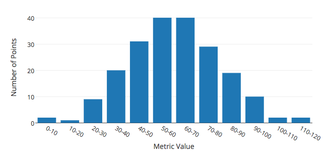
The following table lists the distribution of one metric at successive minutes. The first row of the table contains the distribution illustrated in the figure. The following rows show how the distribution evolves over successive minutes.
| Time (minute) | Distribution (number of points) |
|---|---|
| 1 | [2, 1, 9, 20, 31, 40, 40, 29, 19, 10, 2, 2] |
| 2 | [2, 1, 9, 22, 31, 38, 41, 28, 17, 11, 3, 2] |
| 3 | [1, 2, 10, 21, 31, 39, 40, 29, 19, 10, 1, 2] |
| 4 | [2, 1, 9, 19, 29, 40, 41, 31, 20, 10, 1, 2] |
Histogram Bin Size
Histogram bin size is computed using a T-digest algorithm, which retains better accuracy at the distribution edges where outliers typically arise. In the algorithm, bin size is not uniform (unlike the histogram illustrated above). However, the bin size that the algorithm selects is irrelevant.
Histograms do not store each actual data point value that is fed to it. Instead, histograms store the quantiles calculated from histogram points, which are estimates within a certain margin of error.
Histogram Metric Aggregation Intervals
Tanzu Observability supports aggregating metrics by the minute, hour, or day. Intervals start and end on the minute, hour, or day, depending on the granularity that you choose. For example, day-long intervals start at the beginning of each day, UTC time zone.
The aggregation intervals do not overlap. If you are aggregating by the minute, a value reported at 13:58:37 is assigned to the interval [13:58:00;13:59:00]. If no metrics are sent during an interval, no histogram points are recorded.
Monitoring Histogram Points
You can use ~histogram metrics to monitor histogram ingestion. See the Ingest Rate by Source section of the Tanzu Observability Service and Proxy Data dashboard.